In my last post Bloom Filters: MathMania, we worked through the derivations for optimal number of bits to allocate and the right number of hash functions to use – striking a balance between space, computation, and false positives.
But all of that math rested on one simple assumption: the set of elements going into those derivatios is fixed.
But what happens when it isn’t?
Let’s explore this through the lens of how Bloom filters are used in LSM-based storage engines.
Mutable Memtables: A Headache for Bloom Filters
Memtables are in-memory write buffers in an LSM Tree. Under the hood they are implemented as red-black tree or a skip list both of which are already efficient data structures with decent lookup time of O(log N).
But how about using a Bloom filter on top to make lookup time even more desirable i.e., O(1)? On paper, it sounds attractive - insertion and query in a Bloom filter are just a handful of hash computations. But in practice, it doesn't work out, and the main culprit is changing size.
Bloom filters are tuned to a fixed set size n. Memtables, by contrast, are constantly changing i.e., keys are constantly inserted, updated, and deleted. This drifting set size, causes finely tuned false positive rate and derived space computation thrown out of window:
• Build a Bloom filter for a memtable with 1 million keys.
• A little later, inserts push it to 1.2 million. The carefully tuned false positive rate you started with is now higher than budgeted.
• Or suppose half the keys are deleted. You’re left with a filter that’s oversized, wasting memory.
It’s like buying a fitted shirt for a moving target — sometimes too tight, sometimes too loose, never quite right.
Why Drift Breaks Bloom Filters
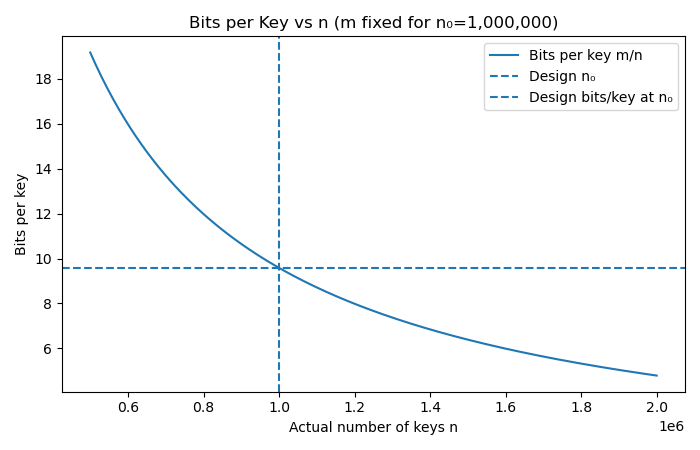
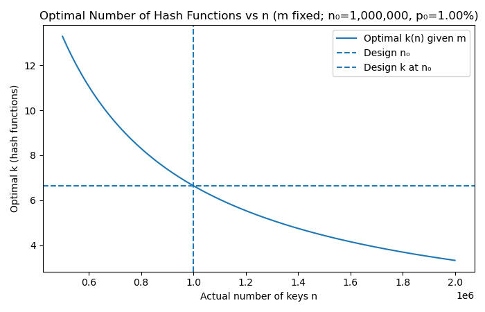
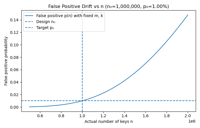
To see why Bloom filters and mutability don’t mix, let’s look at how three core metrics — bits per key, the optimal number of hash functions, and the false positive probability — change as the number of elements n drifts. The following charts make the drift crystal clear:
1.Bits per key \( = \tfrac{m}{n} \)
With m fixed, as n increases, the denominator grows and fewer bits are available per key, resulting in higher false positive rates because the filter becomes “overcrowded.”
2.Optimal number of hash functions (k) \( = \tfrac{m}{n} \cdot \ln 2 \)
As m/n decreases with n, the optimal number of hash functions k also decreases. With too many keys, applying the original k hashes over a crowded bit array just increases collisions instead of helping.
3.False positives (p) \( \approx (1 - e^{-kn/m} )^{k} \)
With m and k fixed at design time, as n grows, the exponent -kn/m becomes larger, which means a larger fraction of the bit array gets flipped to 1. Eventually, almost every lookup “sees” all k bits set, even for keys that were never inserted. Resulting in false positive probability rising above the intended target, drifting away from what you designed for.
Immutable SSTables: The Bloom Filter Sweet Spot
In an LSM Tree, once a memtable is full, it’s flushed to disk as an SSTable (Sorted String Table). And unlike memtables, SSTables are immutable: once written, they never change.
That one property makes all the difference for Bloom filters i.e., the exact number of entries n is known at creation time.
We can compute Bloom filter parameters perfectly: No guesswork. No drift. No “moving target shirt” problem.
Suppose an SSTable has 1,000,000 keys and we want a 1% false positive probability.
Plugging into the formulas:
\( m \approx - \frac{1,000,000 \cdot \ln(0.01)}{(\ln 2)^2} \) \( \approx \) 9.6 million bits (~1.2 MB).
\( k = \frac{9.6 \times 10^6}{1,000,000} \cdot \ln 2 \approx 7 \)
In other words, we can keep the false positives neatly bounded at 1% by:
- Allocating a 1.2 MB bit array, and
- Hashing each key with 7 functions
And since an SSTable never changes, its Bloom filter stays valid for the table’s entire lifetime. When SSTables are eventually merged during compaction, their Bloom filters are discarded along with the old tables and rebuilt fresh for the new SSTable.
Why This Matters
- Reads get faster: SSTables that don’t have the key can be skipped entirely.
- Memory budgeting is predictable: you know exactly how much RAM is needed for filters.
- False positive rate is guaranteed: no drifting as keys are added or removed.
This combination is one reason LSM-based stores (like LevelDB, RocksDB, Cassandra) can scale read-heavy workloads efficiently despite their write-optimised structure.
The Bigger Design Lesson
Immutability doesn’t just make concurrency easier — it also makes probabilistic data structures more powerful.
By freezing data at the SSTable level, LSM Trees let Bloom filters deliver on their mathematical promises: space-efficiency, predictability, and bounded error.